반응표면법기반 강건파라미터설계에 대한 문헌연구: 실험설계, 추정 모형, 최적화 방법
A literature review on RSM-based robust parameter design (RPD): Experimental design, estimation modeling, and optimization methods
Article information
Trans Abstract
Purpose
For more than 30 years, robust parameter design (RPD), which attempts to minimize the process bias (i.e., deviation between the mean and the target) and its variability simultaneously, has received consistent attention from researchers in academia and industry. Based on Taguchi’s philosophy, a number of RPD methodologies have been developed to improve the quality of products and processes. The primary purpose of this paper is to review and discuss existing RPD methodologies in terms of the three sequential RPD procedures of experimental design, parameter estimation, and optimization.
Methods
This literature study composes three review aspects including experimental design, estimation modeling, and optimization methods.
Results
To analyze the benefits and weaknesses of conventional RPD methods and investigate the requirements of future research, we first analyze a variety of experimental formats associated with input control and noise factors, output responses and replication, and estimation approaches. Secondly, existing estimation methods are categorized according to their implementation of least-squares, maximum likelihood estimation, generalized linear models, Bayesian techniques, or the response surface methodology. Thirdly, optimization models for single and multiple responses problems are analyzed within their historical and functional framework.
Conclusion
This study identifies the current RPD foundations and unresolved problems, including ample discussion of further directions of study.
1. Introduction
Starting in the mid- to late-1940s, the Japanese manufacturing industry struggled to survive under extremely limited resources. Many scientists and researchers attempted to revolutionize the manufacturing processes in order to improve the quality of manufactured goods and reduce costs. Taguchi, a Japanese consultant, realized that all manufacturing processes are affected by sources of noise that have significant effects on product variability. Consequently, in the 1950s, Taguchi introduced an important methodology based on statistics to control the quality of products and processes in the design stage; this was popularized in the USA in the 1980s. Taguchi’s methodology is the basic foundation of what is generally named robust parameter design (RPD) or, briefly, robust design.
In this statistical approach to quality control engineering, products and processes are usually considered as a box or system with inputs and outputs (commonly represented by y). Taguchi classified pertinent inputs into two categories: control factors (normally denoted by x) and noise factors (normally denoted by z). Whereas noise factors are difficult or too expensive to control (or potentially even uncontrollable), the control factors can be easily manipulated within the system. The objective of RPD is to select the best combinations of control factors to optimize the quality level of a product by reducing the product’s sensitivity to noise factors. Taguchi designed a number of unique orthogonal arrays (which are essentially balanced fractional factorial designs) to aid in the development of experiments. While noise was treated as a nuisance (blocking) in the traditional design of experimental methods, Taguchi examined the effects of noise factors on experimental designs. The settings of the control factors are contained in an inner array, whereas an outer array is used to contain the noise factor settings for a particular run. This explicit inclusion of noise variables is an important contribution of Taguchi’s (Lucas, 1994). To determine the optimal factor settings, Taguchi considered both the mean and variance of the characteristics of interest as a single performance measure, and used signal theory to derive a number of signal-to-noise ratios (SNRs) from the Taguchi loss function. Among over 60 types of SNR, three are widely used: nominal is best, larger is better, and smaller is better. The appropriate SNRs can be chosen to achieve the optimal control factors x based on the maximization or minimization of some objective function.
Nominal is best
Larger is better:
Smaller is better:
Taguchi’s philosophy received considerable attention from statisticians and researchers, and thus made a remarkable contribution toward the improvement of product/process quality. However, Taguchi’s procedure for solving the RPD problems has been criticized for several shortcomings regarding the orthogonal arrays and SNRs. Firstly, in the experimental design, controllable and uncontrollable factors are placed in two separate arrays (i.e., inner and outer), resulting in more experimental runs (Shoemaker and Tsui, 1991); secondly, the use of orthogonal arrays is rather limited and fails to investigate the interactions between control and noise factors (Myers and Montgomery, 1995). The combination of control and noise factors in a single array is more economical and superior to the orthogonal arrays. Moreover, the arguments for the universal use of SNRs are unconvincing (Vining and Myers, 1990; Yum et al., 2013; Byun et al., 2013). In addition, Taguchi’s method does not exploit a step-by-step method to determine the optimal parameter settings.
Therefore, alternative approaches that are more efficient than Taguchi’s method have been proposed in an attempt to establish a systematic procedure based on his philosophy. A new research trend has derived from the dual response (DR) model based on the response surface methodology (RSM), which was proposed by Vining and Myers (1990). This approach includes two significant contributions: (1) in terms of estimation, the mean and variance of the output responses are considered and estimated as two separate functions of input factors based on the least-squares method (LSM); and (2) in terms of optimization, a robust design model is used to investigate the trade-off between the estimated mean and variance functions. Based on the DR model approach, the second development stage of RPD has three sequential stages: the design of experiments, estimation, and optimization.
RSM is a collection of mathematical and statistical techniques that are useful for modeling and analyzing problems in which the response of interest is influenced by several factors. When the exact functional relationship is not known or very complicated, conventional LSM is typically used to estimate the functional forms of the input response (Box and Draper, 1987; Khuri and Cornell, 1987). To use LSM-based RSM, the basic assumption is that the error terms are independent and normally distributed with constant variance and zero expectation. Unfortunately, this assumption is often violated in practical scenarios. Subsequently, a number of estimation approaches for the unknown model parameters in the mean and variance functions have been proposed, such as weighted least-squares (WLS) (Luner, 1994), Bayesian estimation (Chen and Ye, 2011; Goegebeur et al., 2007), and generalized linear models (Nelder and Lee, 1991). Along with the development of estimation methods for the DR model, the single-response (SR) model based on RSM can also handle the functional relationships between the output responses and both control and noise factors. The interactions between the control and noise factors and the quadratic interactions among noise factors in the SR model have been considered by Myers (1992) and Abate et al. (2007), respectively.
In conjunction with the development of estimation methods, several RPD optimization models have been proposed and extended to determine the optimal factor settings. Using various criteria, these optimization models consider the trade-off between the bias and variance, with examples including the mean square error model (Lin and Tu, 1995), weighted sum model (Cho et al., 1996; Koksoy and Doganaksoy, 2003), fuzzy model (1998), desirability function model (Borror, 1998), and bias-specified model (Shin and Cho, 2005); or between multiple responses, such as the quality loss function model (Ames et al., 1997), dual response-based quality loss model (Romano et al., 2004), lexicographical weighted-Tchebycheff model (Shin and Cho, 2009), and lexicographical dynamic goal programming model (Nha et al., 2013).
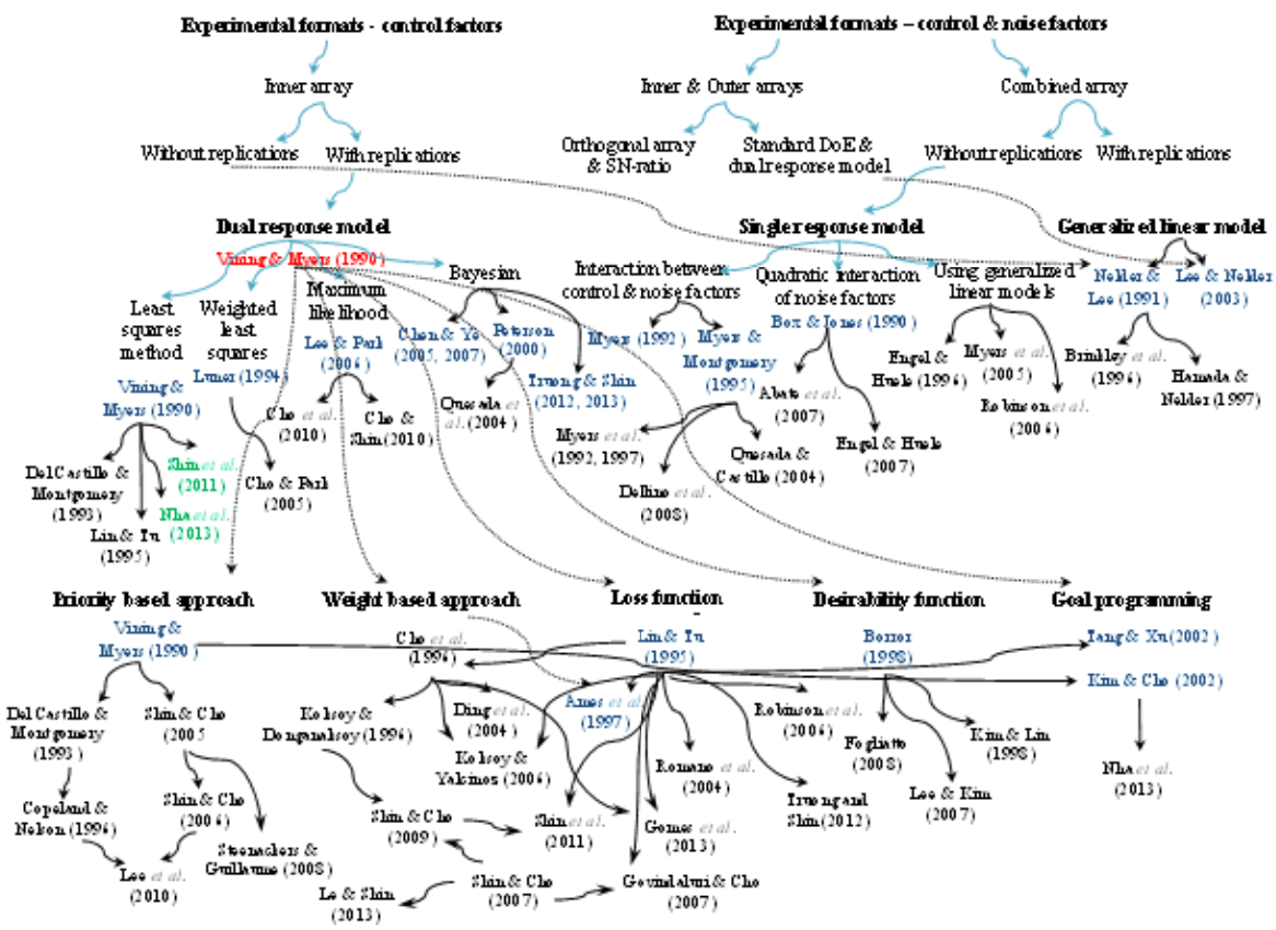
It is more than 30 years since RPD was first introduced, and a variety of solution methods have been proposed to solve the associated problems. Information about the various approaches is scattered throughout the literature and has not yet been fully reviewed in terms of a systematic understanding of the whole RPD methodology. Therefore, the great motivation for this paper is to provide a thorough and systematic discussion of the developments and limitations in the three basic stages of RPD. Firstly, the experimental formats related to both the control and noise factors and to the control factors alone are examined separately. This allows existing problems in the experimental design stage to be discussed in depth. Secondly, two major RPD modeling methods based on RSM, (i.e., SR and DR models) are investigated regarding their simulation of the relationships between the output and control factors both with and without noise. The use of generalized linear models (GLMs) as another technique and the trend of combining RPD with online techniques are also examined. A number of the associated estimation methods (i.e., LSM, MLE, Bayesian approach, and GLMs) reported in the literature are discussed and represented in timeline tables. Moreover, various RPD optimization models based on various criteria for single- and multiple-response problems are deliberated. Numerical examples using these estimation methods and optimization models are briefly discussed in this paper. Finally, based on existing methods, the requirements for future research and further developments in RPD are extensively investigated. As a result, this paper is not only a useful introduction for those new to RPD, but also an important summary of the state-of-the-art for RPD researchers. Figure 1 illustrates an overview of the three basic stages of RPD with their associated classifications. A number of representative studies on both RPD estimation and optimization are shown in Figure 2, along with their corresponding experimental formats.
Existing problems in the design of experiments in various formats are highlighted in Section 2. Section 3 then discusses the estimation methodologies in three different modeling approaches. The development stream of RPD optimization models for single and multiple responses is surveyed in detail in Section 4. Finally, a summary and conclusions close the paper in Section 5.
2. Discussion of experimental formats
Theoretically, the design of experiments is intended to ensure that tests are conducted with deliberate changes by the experimenter regarding the input factors of the product/process so as to obtain information about the nature or phenomenon of the relationship between the input and output variables. As the number of input factors increase, the total number of combinations of factors increases significantly, and the relationships with the output responses become very complicated. In addition, if all experiments are investigated, the overall process becomes both expensive and time-consuming. Obviously, a well-designed experiment is necessary to identify the “vital few” factors that obtain sufficient information about those complex relationships in an effective and economical manner, and then determine the best settings for these factors to obtain satisfactory output functional performance in products/processes.
In practice, some of the process variables or factors can be controlled and some of them are difficult or expensive to control during normal production or under standard conditions. Based on the existing problems, and the available time and cost, a suitable experimental design can be selected to conduct the experiments. The main objectives of the experiments may include the following (Montgomery, 2005):
•Determining which variables have most influence on the response.
•Determining where to set the influential input factors so that the response is almost always near the desired nominal value.
•Determining where to set the influential input factors so that the variability of the response is small.
•Determining where to set the influential input factors so that the effects of the uncontrollable variables are minimized.
In this paper, several experimental formats are discussed and classified into two major categories, namely those including two separate arrays to handle both control and noise factors together and those with a single array to handle control factors only.
2.1. Control and noise factors
In the context of manufacturing, a process is the transformation of input factors or process variables into output responses. The quality of the output products is determined by the variation of the inputs, especially the noise factors. Generally, noise factors are uncontrollable in most actual processes. However, they can be controlled in some specific conditions for the purpose of experiments. In RPD, two popular experimental formats are often used to design the experiments while considering both the noise and control factors.
2.1.1. Experimental formats involving crossed array designs
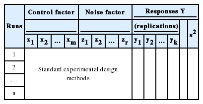
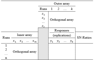
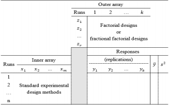
Contrary to the previous work of statisticians, Taguchi incorporated noise factors into the experimental design to consider the influence of uncontrollable factors on the outputs, with the noise factors and their levels specified in a similar manner to those used for control factors. Based on a variety of defined orthogonal arrays, Taguchi proposed a crossed array design consisting of an inner array and an outer array, as presented in Table 1. The inner array contains the control factors and the outer array consists of the noise factors. In Table 1, SNRs are used as a performance measure of the responses. In the crossed array design, each run in the inner array is performed with all combinations of noise factors in the existing outer array, and sufficient information about the interactive effects of control and noise factors on the output factors can be identified quickly. By using orthogonal arrays in the experiments, a number of variables that have the greatest effect on the performance characteristics can be determined. However, not all of the effects of all variables are considered by the orthogonal arrays, because not all variable combinations are examined. As a whole, the orthogonal arrays are useful for screening designs at the beginning of a project. To investigate all combinations of control factors, standard experimental design methods are generally applied to the inner array, and factorial designs or fractional factorial designs are suitable for implementing experiments for the noise factors in the outer array. Normally, the process mean and variance are employed as performance measures of the output responses instead of the SNRs in Table 1. Consequently, another experimental format using combined array designs is demonstrated in Table 2.
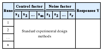
The main limitation of the experimental formats illustrated in Tables 1 and 2 is that the number of replications of the response is dependent on the number of runs of noise factors in the outer array. In addition, the control and noise variables are assumed to be dependent, although in practice, the noise variables have a significant influence on the control variables. Other limitations are that the noise factors are not executed in the estimated mean and variance functions in the experimental format in Table 2, and the SNRs are unable to distinguish between inputs that affect the process mean from those that affect the variance in the experimental format in Table 1.
2.1.2. Experimental formats involving combined array designs
The crossed array designs generally result in a large number of experimental runs, because two separate designs are developed and then combined. Moreover, it is difficult to clarify the nonlinearities in the interactions between the control and noise factors. To overcome the drawbacks of the crossed array designs, Borkowski and Lucas (1991), Box and Jones (1992b), Montgomery (1991), Myers (1991), Shoemaker et al. (1991), Welch and Sacks (1991), Sacks et al. (1989), and Myers et al. (1997) proposed alternative combined array designs in which the control and noise factors are combined in a single array. Considerable time and money can be saved using combined array designs, as they require fewer experimental runs than the crossed array designs. Depending on the replications of the output responses, combined array designs have two typical experiment formats, as represented in Tables 3 and 4.
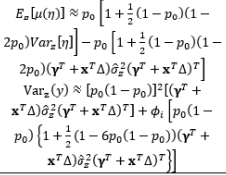
Theoretically, the DR model approach is the fundamental method of modeling the relationship between the input and the responses of interest with replication. However, using the DR method to estimate the mean
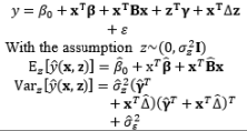
Another experimental format for conducting experiments with the control and noise factors using the combined array design is demonstrated in Table 4. The SR model approach is typically used to obtain estimated functional forms of the responses without replication. Normally, the errors of the noise factors are assumed to follow a normal distribution with zero mean and constant variance
2.2. Control factors only
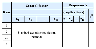
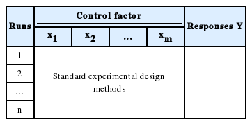
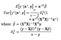
Most experiments and experimental design methods in the literature consider the control factors only. Based on replications of the responses of interest, two types of experimental formats in which the control variables are contained in the inner array are illustrated in Tables 5 and 6. Similarly, the DR model approach is employed to model the response with replication, as presented in Table 5, whereas the SR model method is used in Table 6.
In these experimental formats, the design of experiments is simpler and requires less time than when noise factors are also considered. The limitation of the experimental formats in Tables 5 and 6 is that important information about the interactions between the control and noise factors is missed because the noise factors are not examined in the experiments. Therefore, the final optimal solutions may not indicate the highest degree of accuracy of the problems.
3. Estimation methods
3.1 Dual response model
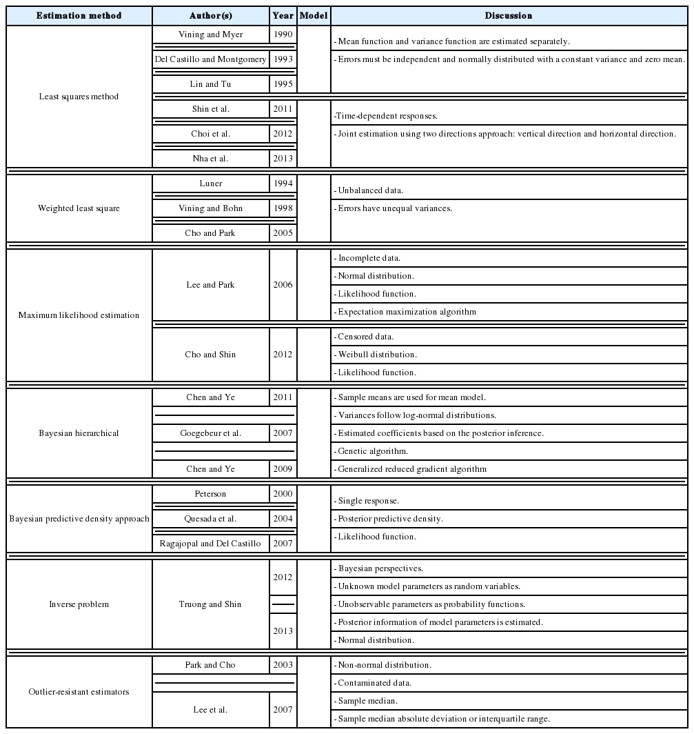
The first attempt to integrate RSM into RPD as an alternative to Taguchi’s method is the DR model approach proposed by Vining and Myers (1990). In the DR framework, the mean and standard deviation of the response are taken as functions of the control factors using RSM and the unknown coefficients in both functions are estimated by LSM. Further intensive studies on the DR model based on LSM are discussed by Del Castillo and Montgomery (1993), Lin and Tu (1995), and Copeland and Nelson (1996). Shaibu and Cho (2009) observed that the accuracy of predictions given by the DR model based on LSM can be increased by using higher-order polynomial response functions instead of the quadratic form in most RPD applications. Shaibu and Cho (2009) employed statistical model selection techniques to choose a pool of factors in the higher-order form. In contrast to these proposals for handling static responses, Shin et al. (2011a), Choi et al. (2012), and Nha et al. (2013) developed joint estimation methods using a two-directional (vertical and horizontal) approach to examine time-oriented responses in the pharmaceutical field.
The DR model approach using LSM to estimate the model coefficients is the basic method, and is widely used in many RPD situations. Two basic assumptions of LSM are that all the data follow normal distributions and that random error terms are normally distributed with constant variances and zero means. Unfortunately, these assumptions are often violated in practical scenarios, meaning that the Gauss–Markov theorem is no longer valid. Consequently, methods such as transformation, WLS, MLE, and Bayesian techniques are often applied to achieve valid estimations in industrial applications. The most popular method of transforming the dependent variable used to fit the model is the Box–Cox transformation, or power transformation, which has been applied in RSM by Lindsey (1972).
By analyzing the Roman-style catapult study, a well-known example in RPD, Luner (1994) found that each of the input factors has a different impact on the output responses, and proposed the WLS method to estimate the model coefficients in the mean and variance functions. Moreover, Cho and Park (2005) generalized a number of unbalanced data cases to use the WLS method in the DR model, such as an unequal number of replicates at each design point, some treatment combinations being more expensive than others, some treatment combinations being more interesting, and some missing experimental data.
To implement RSM using LSM, the data are commonly full sets of observations. In many industrial applications, however, partial sets of observations coexist with fully observed sets. Datasets consisting of both partially and fully observed records are commonly called incomplete (Lee and Park, 2006). For incomplete data, Lee and Park (2006) incorporated expectation-maximization and the MLE method into the DR model approach under the assumption that the observations are normally distributed. In other real-world situations, the experimental data obey non-normal distributions, for instance, censored data often follow the Weibull distribution. Cho and Shin (2012) applied the MLE method to estimate the mean and variance of pharmaceutical time-oriented data, that is, the censored Weibull data.
In the DR model based on LSM, the estimated variance can have a negative value, even if the true mean variance is positive throughout the region of interest. If the response at a point with a negative predicted variance happens to be the optimum under a certain criterion, it would be difficult to explain the process performance at this point (Chen and Ye, 2011). To overcome this drawback and attain meaningful optimal solutions, Chen and Ye (2011) introduced the Bayesian hierarchical approach, which is suitable for the hierarchical structure of DR models, and two mathematical techniques based on a genetic algorithm and the generalized reduced gradient algorithm. This Bayesian hierarchical approach was extended to partially replicated designs by Chen and Ye (2009). Goegebeur et al. (2007) also utilized the Bayesian hierarchical approach based on Gibbs sampling and the Metropolis–Hastings algorithm to determine the coefficients in the DR model. Another Bayesian approach for determining the mean and variance functions of the response of interest is to consider the uncertainty in the parameter estimates given by the Bayesian predictive density function, an approach proposed by Peterson (2000), Quesada et al. (2004), and Ragajopal and Del Castillo (2007). In addition, Ragajopal and Del Castillo (2005) introduced the Bayesian model averaging method to optimize the posterior predictive density function.
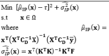
Based on Bayesian principles, Truong and Shin (2012, 2013) integrated the inverse problem (IP) into RPD in an attempt to relax the normality requirements of LSM-based RSM. A basic review of IP theory and the application of IPs to model parameter estimation can be found in Tarantola (1987, 2005). In this RPD estimation method, two sequenced modeling steps (i.e., forward and inverse) are conducted after the parameterization of the system. Truong and Shin (2013) assumed that both the process mean and variance of the responses follow normal distributions, whereas an earlier study (Truong and Shin, 2012) assumed that the observed variances obey the Chi-square distribution.
In all of the above RPD estimation methods, the sample mean and sample variance are used to fit the process mean and process variance functions, respectively. For non-normal data and/or contaminated data, Park and Cho (2003) and Lee et al., (2007) proved that the use of the sample mean and sample variance to model the dual response surface model is inappropriate. Instead, they proposed the median and median absolute deviation or interquartile range as good alternatives to the mean and variance, respectively, especially in the case of Laplace, logistic, and Cauchy distributions. To estimate these “mean and variance” functions, Park and Cho (2003) derived outlier-resistant estimators. However, it is well known that these estimators are inefficient in the case of a normal distribution. Therefore, Lee et al., (2007) recommended other highly efficient and resistant regression methods, such as Huber’s proposed 2M-estimation and resistant regression based on MM-estimation. Furthermore, Ch’ng et al. (2007) applied the three-stage MM-estimator procedure defined by Yohai et al. (1991) to estimate the mean and variance functions. Huber’s proposed 2M-estimation and resistant regression based on MM-estimation are described in Huber (1981) and Yohai et al. (1991), respectively. The existence and classification of outliers in the context of regression models are explained in Montgomery et al. (2001). The estimation methods used in the DR model are summarized in Table 7.
3.2. Single-response model
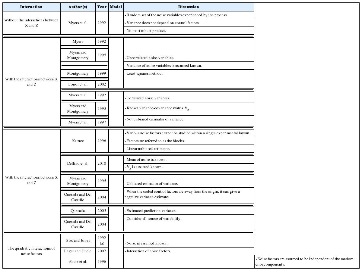
In combined array designs, the interactions between control and noise factors and among the various noise factors are investigated, and the resulting information about their effects on the output responses is exploited. From this information, the output responses can be modeled as a function of both control and noise factors using the SR model approach based on RSM. Regarding this modeling trend, Myers et al. (1992) commented that the methods for modeling the mean response have been thoroughly investigated because the mean is not related to the noise factors in the function, the attention directed toward variance modeling is considerable, and the model for the process variance is likely to be even more important than the model for the mean in RPD problems. The fundamental element of all estimation methods in this modeling direction relies on the assumptions made about the noise factors. Most modeling methods assume that the noise factors are either known or can be estimated well. In addition, the random error terms are also assumed to be NID(0,
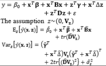
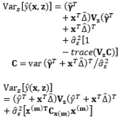
In the literature, the SR model including the full quadratic form of the control factors, the main effects of noise, and the interactions between the control and noise factors is probably the most widely employed model for illustrating the output response as a function of the control and noise variables. Myers (1991), Myers and Montgomery (1995), Montgomery (1999), and Borror et al. (2002) assumed that the noise factors are uncorrelated and that their variance is known (i.e., (
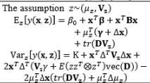
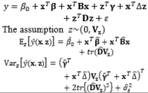
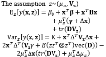
The full and general form of the SR model approach proposed by Box and Jones (1992a) consists of the quadratic form of control factors and all interactions between the control and noise factors as well as those among the noise factors. To estimate the process mean and variance functions in this situation, Engel and Huele (2007) applied LSM with the assumption that z~(0, Vz). Another extension of the general SR model approach was reported by Abate (1995) and Abate et al. (1996) based on the assumptions that the noise factors are correlated and the mean value of the noise factor is not equal to zero (i.e., ~(µz, Vz)). The trace and Kronecker product are used to determine the estimated mean and variance functions. The classification of all models in the SR approach and the associated discussions of each model are outlined in Table 8.
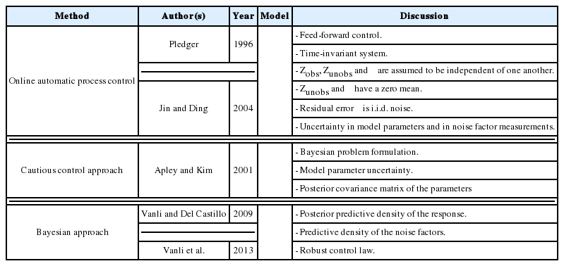
Most RPD methods reported in the literature are used to identify appropriate settings for the control factors in the offline design stage, thus reducing the process and product variability based on the assumption that the noise factors are well known or can be controlled in laboratory environments. The offline application of RPD may be ineffective if there are noise factors with strong autocorrelation or non-stationarity, or if the noise factors can be measured during production (Pledger, 1996; Dasgupta and Wu, 2006). This has resulted in a new tendency whereby RPD is combined with online control techniques or schemes to measure the noise factors during production and give better performance, namely online RPD. For the case of strong noise factors in the process, Joseph (2003) developed a general RPD methodology to find the optimal offline settings of control factors in the simultaneous presence of a feed-forward control law for a single additional control factor in single-response and multiple-target systems. Similar to Joseph (2003), Dasgupta and Wu (2006) developed an RPD framework with a discrete proportional-integral feedback control scheme based on a single experiment. They used a performance measure modeling approach to model the output as a function of the input variables. Jin and Ding (2004) classified noise factors into two sets: (i) observable noise zobs and (ii) unobservable noise zunobs. Using the SR model based on RSM, Pledger (1996) and Jin and Ding (2004) incorporated feed-forward control into RPD so that the controllable factors could be adjusted online based on in-process observations of noise factors. The online automation of process control using regression models discussed by Jin and Ding (2004) can also be applied to the uncertainty in the model parameters and the uncertainty in the measurements of the noise factors. Along this line, Apley and Kim (2011) developed a cautious control approach, a terminology used previously for quality control (Apley and Kim, 2004), that uses adaptive feedback to take model parameter uncertainty into account via the posterior parameter covariance. In contrast to the known noise variables assumption in the SR model approach of offline RPD, Tan and Ng (2009) investigated the effects of random sampling errors in the noise factors on the estimated mean and variance models, and proposed a framework for designing a combined array experiment and a new sampling method that estimates the mean and covariance of the noise factors. To reduce uncertainty in the response model and noise model parameters, Vanli and Del Castillo (2009) proposed a new Bayesian online RPD approach that calculates the posterior predictive density of the responses using a Bayesian response model robust control law and determines the predictive density of the noise factors through a Bayesian response and noise model robust control law. This is an extension of the Bayesian predictive approach to offline RPD used by Miro-Quesada et al. (2004) to derive closed-form control rules for use in online RPD. However, the posterior distributions of the model parameters are obtained from offline data and are not updated with online observations during production. Therefore, Vanli et al. (2013) extended this approach to the adaptive case in which model estimates are updated with online observations by using Bayesian regression and time series models. This allows the operators to re-compute the settings of the control factors online to better account for autocorrelation and non-stationary behavior in the noise factors. An overview of the methods used in online RPD with online control techniques and the associated discussions is presented in Table 9.
The SR model approach introduced by Myers et al. (1992) is probably the most popular method of modeling the response variables as a function of the control and noise variables for both online and offline RPD in quality improvement applications. The generalized linear modeling in the next subsection is a partial extension of this SR model method.
3.3. Generalized linear models
Along with the development of the DR and SR modeling methods for determining the functional form of the input and output factors in RPD, GLMs have also been applied to RPD modeling. There are two distinct trends in the application of GLMs to RPD: GLMs as an extension of the SR model proposed by Myers et al. (1992), and GLMs as an alternative response modeling approach. Whereas Myers et al. (1992) were the first to suggest the former, Nelder and Lee (1991) pioneered the use of the latter. The theory of GLMs has been widely discussed in the literature.
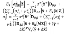
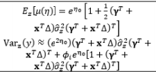
In the SR model approach, the residual variation
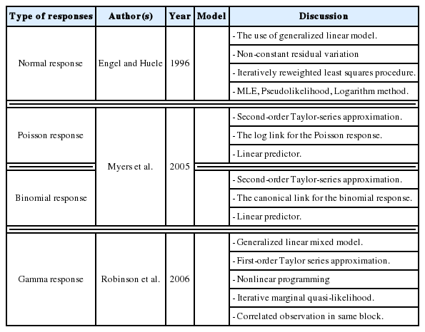
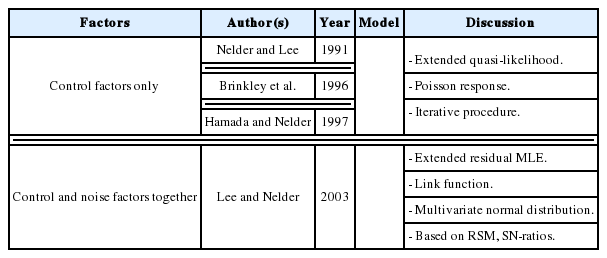
In early attempts to integrate GLMs into RPD, Nelder and Lee (1991) modeled the mean and dispersion as functions of control variables with a Poisson response. In terms of joint modeling for the mean and dispersion, extended quasi-likelihood algorithms were used to estimate the parameters model with a four-step-iterative procedure. Instead of transforming the non-normal data and analyzing them by standard normal methods, Hamada and Nelder (1997) proved that GLMs can be used as a natural alternative for a variety of data with the same iterative strategy. Brinkley et al. (1996) combined GLMs with nonlinear programming to obtain optimal solutions in a case study on circuit board quality improvement with Poisson quality characteristics, whereas Paul and Khuri (2000) used ridge analysis within the framework of GLMs to find the optimal operating conditions for the exponential family. Along the same lines, the GLM response functions were developed explicitly with the non-constant dispersion parameter ɸi in log form by Engel (1992). In addition, three main components in GLMs, namely the location (fixed) effects, dispersion effects, and random effects, were jointly estimated as the parameters related to control, noise, and random factors using residual MLE with a general mixed model by Wolfinger and Tobias (1998). The consolidation of joint modeling for the mean and dispersion in GLMs and the four main advantages of the GLM approach in RPD were discussed by Nelder and Lee (1998).
In another attempt to extend the GLM framework as a tool for solving RPD problems, Lee and Nelder (2003) considered the mean and dispersion as functions of both control and noise factors. The authors represented a broad framework of RPD approaches based on interpreting RSM, SNRs, and data transformation through the GLM structure to give joint GLMs for the mean and dispersion. The literature on GLMs is broadly covered by Myers and Montgomery (1997), Hamada and Nelder (1997), and Myers et al. (2002). An overview of the GLM approach used as an alternative modeling methodology in RPD is presented in Table 11.
4. RPD optimization models
The key purpose of the RPD optimization stage is to identify appropriate settings for the process design variables. Such settings are generally those that minimize the performance variability and the deviation from some nominal value of a quality characteristic of interest. The development of RPD optimization models and approaches can be classified into three important milestones. Originally, in the early stages of RPD, the two-step model of Taguchi was used to determine the nominal best case. In this approach, the control factors are classified into two main groups: (i) the variability control factors, which affect the variability and probably the mean of a process, and (ii) the target control factors, which only affect the mean of a process. To construct this optimization model, the variability control factor settings that maximize the SNRs must first be established. The mean response to the desired target value is then adjusted by changing the target control factors. The disadvantages of the two-step model lie in the orthogonal array and SNRs, as discussed in previous sections.
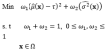
The second development stage of RPD optimization models originates from the DR model approach proposed by Vining and Myers (1990), in which the estimated mean and variance functions are considered to achieve optimal solutions. The priority criterion is used in the optimization formula to keep the process mean at the customer-identified target value, while the estimated variance function is minimized. However, Del Castillo and Montgomery (1993) and Copeland and Nelson (1996) pointed out that the technique used by Vining and Myers (1990) to solve the RPD optimization problem may not always produce local optima, and that better RPD solutions could be achieved using standard nonlinear programming techniques such as the generalized reduced gradient method and the Nelder–Mead simplex method. Kim and Lin (1998) used fuzzy logic techniques to modify the DR model proposed by Vining and Myers (1990). The estimated mean and variance functions are considered simultaneously based on the member functions in fuzzy set theory. The fuzzy optimization model is based on the L¥ norm. Other extensions of the DR model include the prioritized models proposed by Kim and Cho (2002) and Tang and Xu (2002) based on the idea of goal programming. To specify the upper bound of the process bias and variance, Shin and Cho (2005, 2006) proposed bias-specified and variability-specified models by applying the e-constraint method to the process bias and process variance, respectively.
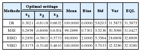
In terms of optimization, the DR model may provide a considerably large variance in some cases, as the process variability is minimized while the process mean remains at the preferred value. According to the illustrated example in Lin and Tu (1995), the process variance can be reduced significantly when some slight deviation from the target value of the process mean is allowed. Hence, Lin and Tu (1995) proposed the mean square error (MSE) model to consider the process bias and process variability simultaneously in the RPD optimization problem. The MSE model proposed by Lin and Tu (1995) is another significant development stage of RPD optimization models. Based on the MSE model, a number of extended approaches have been developed to consider the trade-off between the bias and variance. Steenackers and Guillaume (2008) combined the MSE model and the bias-specified model proposed by Shin and Cho (2005) to determine the appropriate compromise solution. Cho et al. (1996) considered the basic idea of relative importance between the process bias and process variance in the MSE model by suggesting a weighted sum model. Using the joint optimization of the mean and standard deviation functions, Koksoy and Doganaksoy (2003) provided a more flexible means by which decision makers can generate alternative solutions to the DR model and MSE model using the concept of a weighted sum. Along the same lines, Ding et al. (2004) utilized the convex combination of the estimated mean and variance functions to transform the multiple response functions into a single objective function. Different weight values were assigned to two response functions to plot the Pareto frontiers and minimize the expected loss in the weighted sum model proposed by Ding et al. (2004). Other extensions of the MSE model include the generalized linear mixed models proposed by Robinson et al. (2006) and the IP model proposed by Truong and Shin (2012), which used generalized linear mixed models and the IP estimation method to estimate the mean and variance functions, respectively. To consider the bi-objective optimization of the process bias and process variance, Shin and Cho (2009) suggested a lexicographical weighted-Tchebycheff model consisting of the lexicographical order technique and the assigned weighting method between them in terms of the L¥ norm.
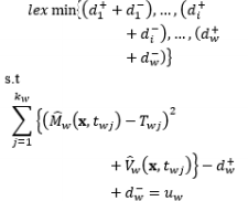
To handle multiple-response quality characteristics optimization problems, several methods have been developed using the concept of RPD. The weighting criterion was used to consider the trade-off between multiple responses in the quadratic quality loss function proposed by Ames et al. (1997). The process mean and variance functions were not employed in this model. Based on the SR model approach, Romano et al. (2004) solved multiple-response optimization problems through the DR-based quality loss model with a constraint involving limits on the mean and variance of individual responses. Contrary to the quality loss function, the desirability approach is used to convert the multiple response functions to the same scale. Borror (1998) used the desirability function model with equal weight values assigned to the mean and variance response surfaces to solve the single-response RPD optimization problem, whereas Fogliatto (2008) combined the desirability function approach with the Hausdorff distance technique to identify the response outcomes that are closest to a target profile. Additionally, the idea of constructing and solving RPD problems with time-series and multiple responses has recently been considered. Nha et al. (2013) proposed a lexicographical dynamic goal programming model using the same-name approach to implement the time-series and multiple responses within the pharmaceutical environment. Goethals and Cho (2010) considered the time-oriented dynamic characteristics problem in terms of economics by integrating a cost mechanism and quality loss approach to a given process across a time profile.
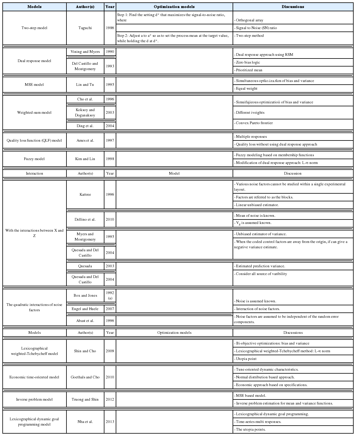
In addition to considering the trade-off between the mean and variance functions, the MSE model can be used as a criterion to compare multiple-response quality characteristics. In the weighted sum approach based on the MSE concept proposed Koksoy (2006) and Koksoy and Yalcinoz (2006), the weights are assigned to the individual MSE functions of each response. For this highly nonlinear or multimodal problem, Koksoy (2006) and Koksoy and Yalcinoz (2006) utilized the NIMBUS algorithm and a genetic algorithm based on arithmetic crossover, respectively, to solve the proposed formulation. Although the weighted sum method can generate efficient solutions for convex multi-objective problems, it cannot, in general, find all efficient points of non-convex problems (Tind and Wiecek, 1999). To overcome this drawback, Shin et al. (2011b) developed a lexicographical weighted-Tchebycheff method based on the MSE term to determine the efficient solutions of a non-convex Pareto frontier in RPD multiple-response optimization problems. However, the correlations between multiple responses are ignored in most formulations. In an attempt to consider the multiple correlated characteristics in the RPD principle, Govindaluri and Cho (2007) employed the Tchebycheff metric-based compromise programming method with the MSE of individual quality characteristics consisting of the mean, standard deviation, and covariance functions. Gomes et al. (2013) identified the drawback of the method proposed by Govindaluri and Cho (2007) based on the computation of a covariance response surface, and developed weighted multivariate MSE model using principle component analysis to obtain the optimal solutions of multiple correlated responses presenting different degrees of importance. The different RPD optimization models reported in the literature are summarized in Table 12.
5. Summary and conclusions
In this paper, the three main stages of robust design have been reviewed in terms of several important aspects. Various experimental formats have been discussed based on the use of control factors only or noise factors and control factors together. The remaining problems in the experimental formats correspond to the noise factors. The modeling the functional relationship between the responses and input factors, including the DR model approach, the SR model approach, and GLMs with various estimation methods, have been discussed. The modeling of time-dependent and multiple responses covers a wide range of practical situations, and requires further exploration in future studies. In addition, this stage of RPD has been investigated more thoroughly because of the uncertainty and accuracy associated with existing modeling methods. The application of online RPD to deal with the noise factors is also an interesting future direction. In addition to the SR optimization models, many approaches have been proposed for multiple responses. The priority and weight criteria are often considered in the proposed optimization models. RPD optimization models have been widely studied. Further considerations could be given to the combination of the priority and weight between the bias and variance, or between multiple responses.
Acknowledgements
This work was supported by the National Research Foundation of Korea (NRF) grant funded by the Korea government (MSIP) [grant number NRF-2014R1A2A1A11049845].

