Article information

Trans Abstract

1. Introduction

Supply chain management refers to harmonized decision making and integrated activities between a firm and other independent business entities in its supply chain. The supply chain contracting decisions for perishable products arise from the notion that operations and supply chain management should be within the larger picture of the business model. This perspective has led managers to recognize that supply chain contracting decisions should be integrated into operational inventory decisions to improve the company’s overall profits. Many researchers have studied a variety of strategic models where profits can be maximized under environmental uncertainties.

A sustainable supply chain is known for its economic and environmental aspects. Uncertainty in a supply chain leads to additional costs. The burden of this additional cost should be resolved through resource efficiency and improved supply chain profits. In this research, we attempt to derive a strategy to achieve efficient resource utilization through supply chain contracting and maximize the supply chain’s profit via supply chain coordination.

The performance of a supply chain diminishes when one or more players in the chain focus on optimizing their own profits. A supply chain contract, therefore, is a coordination system that integrates and incentivizes all the players in the supply chain (Wang 2002). A revenue-sharing contract is an effective way to coordinate between buyers and suppliers. In this context, the primary objective of this study is to investigate whether yield management for perishable products can achieve the goal of supply chain coordination between a single buyer and a single supplier under a variety of environmental conditions. In particular, it investigates: (1) whether yield management can achieve cost reduction under a variety of realistic business conditions, (2) the impact of demand variation on supply chain coordination, (3) the effect of differential cost structures of the buyer and the supplier on supply chain coordination, and (4) the impact of yield rate on supply chain coordination.

Existing literature proposes optimizing the supply chain design for perishable products through the physical supply process (Borumi, Bourtemburg, Horton, and Ladadie, 1986; Ahumada and Villalobos, 2009). As supply chain theory has developed, various types of uncertainties have been considered for establishing a cooperative supply chain (Ahumada and Villalobos, 2009). However, it has still not been applied to existing management science techniques (Ahumada and Villalobos, 2011; Ahumada, Villalobos, and Mason, 2012). In this study, we propose a simulation model that takes into account demand and yield uncertainty for a supply chain contracting model. The efficiency of revenue-sharing contracts has been confirmed by many studies (Wang, 2002; Cachon and Lariviere, 2005). We propose a solution to the yield uncertainty of perishable products under uncertain market demand in a revenue-sharing contracting model (Wells and Singh, 1989; Kazaz and Webster, 2011).

This paper is organized as follows. The important literature was reviewed in Section 2, followed by a description of the supply chain coordination model in Section 3. In Section 4, we report the experiment design and analytical results and summarize the major findings. The paper concludes with a discussion on the limitations and future directions of the research.

2. Literature review

Coordination plays an important role in enhancing the competitive advantage of a supply network and significantly reducing overall cost and uncertainty, while also making the supply chain environmentally and economically sustainable (Chong, Hong, Lee, and Kwon, 2018). For green products especially, participation of all players at every stage of the supply chain is essential to optimize the entire chain (Beske and Seuring, 2014). Yoon and Jeong (2017) studied a sustainable supply chain by supply chain contracting and Hämäläinen et al. (2017) suggested the cost aggregation of a sustainable supply chain to improve coordination in the chain. Downward substitution strategy is a way to achieve resource efficiency. Maddah et al. (2009) suggested using a mathematical formula to arrive at the optimal order quantity in both the EOQ and the classic newsvendor model.

Perishable products are particularly challenging to manage because of the uncertainty about the state of the product right from the production stage up till delivery to the consumer (Baek, Son, and Lim, 2018; Kwon and Hong, 2018). Borumi, Bourtemburg, Horton, and Ladadie (1986) have focused on the operational planning of agricultural products on the supply chain. Both Ahumada and Villalobos (2009) and Borodin, Bourtembourg, Hnaien, and Ladadie (2016) have conducted research on the existing literature on the supply of perishable products. Ahumada and Villalobos (2009) investigated the uncertainties in the supply chain of agricultural products, a vast research area, yielding both research methods and various types of uncertainty.

Blackburn and Scudder (2009) studied strategic supply chains and suggested a design that would maximize the commodity value of perishable products over time. Ahumada and Villalobos (2011) presented short-term strategies for harvesting and distributing perishable products using mixed integer programming to derive optimal operational planning. Ahumada, Villalobos, and Mason (2012) proposed a stochastic model for the production and distribution of fresh agricultural products and sought to derive the optimal supply chain strategies taking into account uncertainties in the supply chain.

Studies on uncertain yields in the supply chain are as follows. Wells and Singh (1989) addressed inventory issues for perishable products by investigating yield uncertainty and analyzing the effect of time, temperature, and inventory display on the yield quality. Kazaz and Webster (2011) analyzed the effects of yield on price and production planning under production uncertainty in terms of yield.

Supply chain contracting is an efficient way to increase coordination between buyers and suppliers. These contracts offer incentives to both buyers and sellers that have integrated supply chains (Wang, 2002). Supply chain contracts provide mathematical solutions to optimize the entire supply chain. Cachon and Lariviere (2005) demonstrated that a revenue-sharing contract can improve coordination in a supply chain.

There are also various studies that compare revenue-sharing contracts based on wholesale prices. Gerchak et al. (2006) demonstrated that in the video rental industry, supply chain coordination is possible through revenue-sharing contracts, taking product sales and product recovery into account. Ouardighi and Kim (2010) conducted a study to compare wholesale price contracts and sales-sharing contracts in horizontal competition. Ai et al. (2012) conducted a comparative study of contracts for retail competition in uncertain market conditions. These studies have demonstrated the need for a collaborative supply chain by demonstrating that a centralized supply chain provides greater benefits than a decentralized one.

3. Supply chain contracting model with yield uncertainty

Assume there are two firms, a manufacturer and a retailer, that follow a fixed-price newsvendor model in a supply chain. The items produced/purchased are of different qualities. We consider yield rate as perfect quality and imperfect quality. Before a single selling season, the manufacturer and the retailer need to decide the optimal order quantity for a given environment by entering into a wholesale price contract. To achieve supply chain coordination, the revenue-sharing contract with downward substitution seeks to maximize the entire supply chain’s profit.

Given that there are two quality grades, retail prices (p₁, p₂) and the wholesale price (ω) are fixed; the order quantity (Q) is the decision variable that simultaneously takes into account uncertainty of demand (D) and yield (α). In the wholesale price contract, the profit of the entire supply chain (π_wt) will be given by the equation:

and the profits of the manufacturer (π_wm) and the retailer (π_wr) will be given by:

In the same environment, the revenue-sharing contract finds the optimal revenue-sharing ratio (Φ) and the optimal wholesale price (w_r) between the manufacturer and the retailer. Together, the optimal revenue-sharing ratio (Φ) and wholesale price (w_r) will determine the optimal order quantity (Q) and the profits of the supplier and the buyer. At this time, the profit (π_rt) of the entire supply chain will be given by:

And the profits of the manufacturer (π_rm) and the retailer (π_rr) will be given by:

We analyzed the efficiency of a revenue-sharing contract and a wholesale price contract considering demand uncertainty and yield uncertainty, profit maximizing ratio, and success ratio. The implications for environmental variation were derived through a comparative analysis between the wholesale price contract and the revenue-sharing contract.

4. Computational Analysis

In this section, we present the computational analysis of the solutions obtained from the supply chain contracting model equations provided in the previous section. The main objective of the computational analysis is to understand the impacts of yield uncertainty and other experimental factors (demand variation and profit sharing ratio) on total profits. Note that profits will be maximized at the optimal order quantity level. Thus, understanding the dynamics under a variety of environmental conditions helps evaluate the effectiveness of a firm’s inventory strategy.

The most complex method to evaluate conceptually is the Monte Carlo simulation (Lee et al., 2016). We performed simulations to give us the results of an optimized supply chain within the environment defined by the experimental factors and parameters. The experimental factors are: 1.) the contract (2 types), 2.) demand variation (3 types), 3.) revenue-sharing ratio (10 types), and 4.) yield rate for perfect quality (7 types). Prior to this study, discrete analysis was carried out by deviating the feasibility of simulations under the experimental environment.

In this study, a total of 420 orthogonal experimental groups (2 × 3 × 10 × 7) were analyzed. The number of simulation repetitions in each management environment was 300 times, and the data on the past demand for simulations are based on the average of the demand generated in the 30th time used in the warm-up period. The input variables and experimental conditions are summarized in <Table 1>. In this study, the salvage value (s) was considered zero (0).

Table 1.

Input Parameters and Experimental Conditions

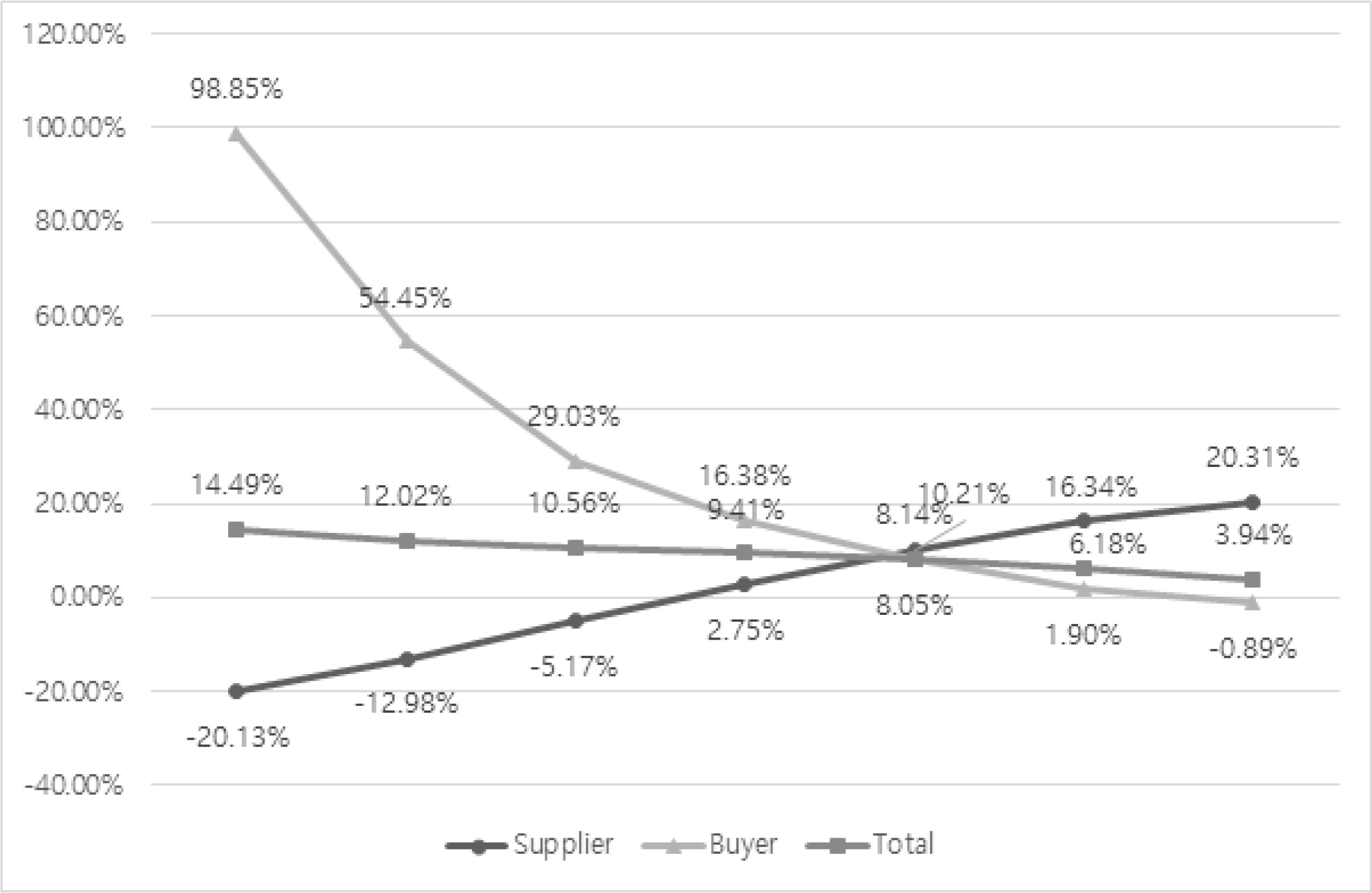
<Table 2, Figure 1>, <Table 3, Figure 2>, and <Table 4> show the change in the overall profit of the supply chain for each management environmental variable.

Table 2.

The change in profit maximizing ratio for demand variation (σ) and revenue-sharing ratio (Φ) (α = 0.7)

Figure 1.

The change in profit maximizing ratio for demand variation (σ) and revenue-sharing ratio (Φ) (α = 0.7)

Table 3.

The change in profit maximizing ratio for demand variation (σ) and yield (α) (Φ = 0.65)

Figure 2.

The change in profit maximizing ratio for demand variation (σ) and yield (α) (Φ = 0.65)

Table 4.

The change in profit maximizing ratio for yield (α) and revenue-sharing ratio (Φ) (σ = 0.2)

In each table, the bold type indicates an increase in profits for the manufacturer, the retailer, and the supply chain as a whole. <Table 2, Figure 1> shows the change in profit ratio for demand variation (σ) and revenue-sharing ratio (Φ) at α=0.7. As demand variation (σ) increases, the increase in the profit of the total supply chain shows "high risk, high return". As revenue-sharing ratio (Φ) increases, the profits of the manufacturer gradually decrease, while the profits of the retailer gradually increase, and this change is linear. It can be seen that the optimum decision interval is one in which the profits of both the manufacturer and the retailer increase, and the profit of the entire supply chain increases. Revenue-sharing contracts offer more profits than wholesale price contracts suggesting that analysis can provide optimal decision-making for supply chain coordination.

<Table 3, Figure 2> shows the change in the profit maximizing ratio for demand variation (σ) and yield (α) at Φ=0.65. As the quality of yield increases, the profits of suppliers appear to increase. This is because better quality products can command higher prices. On the other hand, as the quality of yield increases, the retailer's profits decrease, which is due to the relationship between retail price and cost. The change in profit maximizing ratio for yield (α) and revenue-sharing ratio (Φ) at σ=0.2 is shown in <Table 4>. It can be seen that there is an interval for optimal decision, and the implication can be derived from the yield.

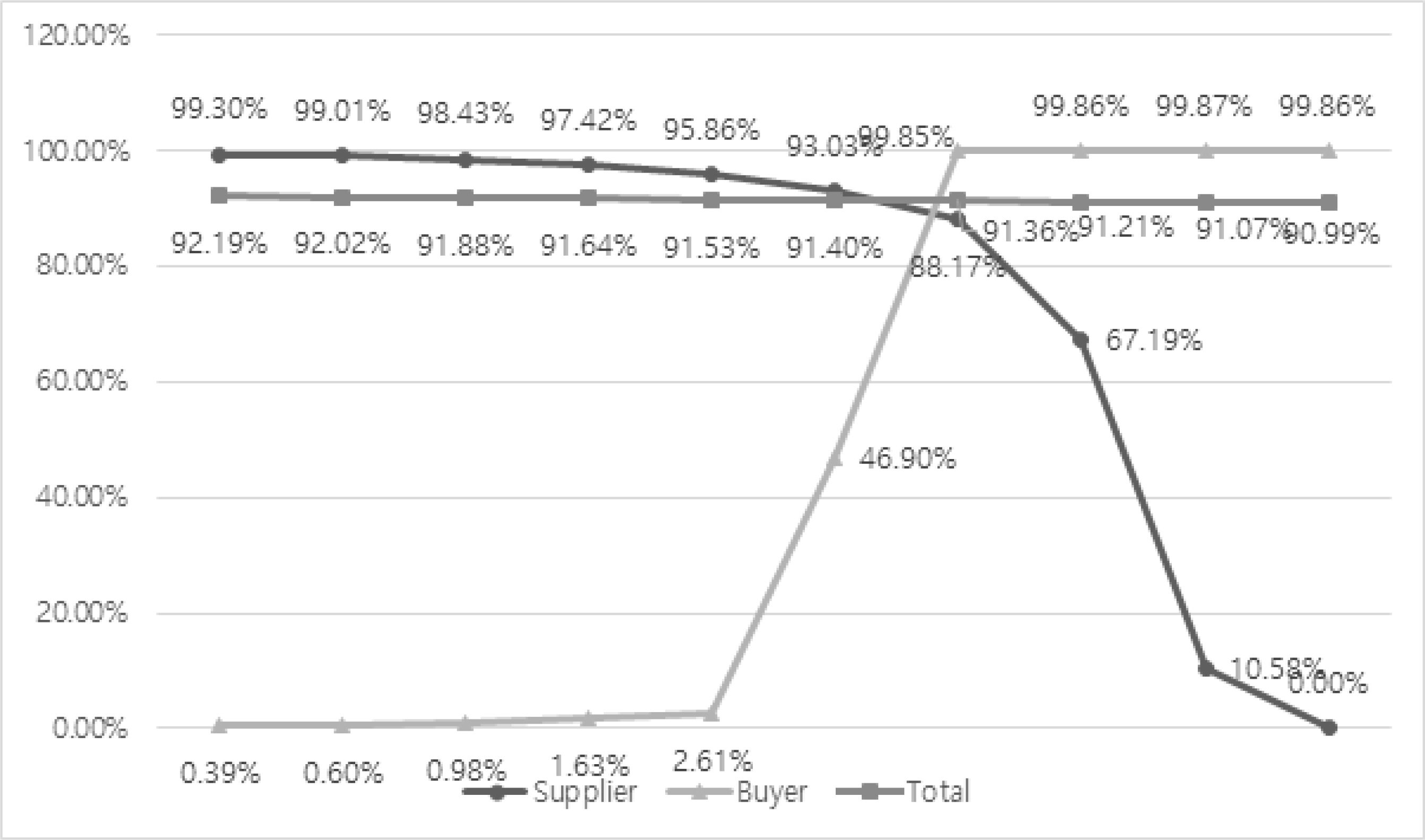
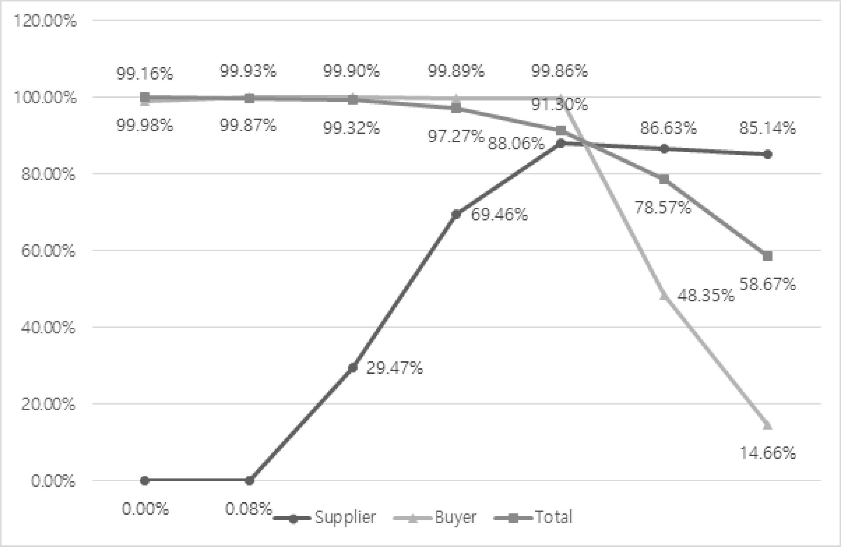
<Table 5, Figure 3>, <Table 6, Figure 4>, and <Table 7> show the change in the success ratio of the supply chain for each environmental variable. Success rate is expressed as the profit increase in the revenue-sharing contract compared to the profit increase in the wholesale price contract. The revenue-sharing contract is not excellent in all circumstances. Therefore, it is necessary to analyze the success rate together with the results of the changes in the profit maximizing ratio. We can see that there is an optimal decision interval in the changes of the profit maximizing ratio, but we need to decide by checking the overall success rate as well. For example, when we look at the success rate while increasing the profits, there is an area where the success rate is less than 60%. Therefore, it is necessary to plan considering both the increase in profits and the success rate of the contract method.

Table 5.

Change in success rae for demand variation (σ) and revenue-sharing ratio (Φ) (α = 0.7)

Figure 3.

Change in success rae for demand variation (σ) and revenue-sharing ratio (Φ) (α = 0.7)

Table 6.

Change in success rate for demand variation (σ) and yield (α) (Φ = 0.65)

Figure 4.

Change in success rate for demand variation (σ) and yield (α) (Φ = 0.65)

Table 7.

Change in success rate for yield (α) and revenue-sharing ratio (Φ) (σ = 0.2)

5. Conclusion

In this paper, we suggest a supply chain contracting model that takes into account the uncertainty in market demand and yield quality of perishable products. We found that a revised revenue-sharing contracting model is more efficient than the wholesale price contract model and allows all members of the supply chain to achieve higher profits.

The experimental findings and their managerial implications can be summarized as follows. First, a strategic approach that includes demand and yield uncertainty helps improve the efficiency of resource utilization. As a result, if there is a supply chain contracting model that offers more profit than wholesale price contracts, it can provide optimal decision-making for supply chain coordination. Among the strategic alternatives, a revised revenue-sharing contract can help increase the efficiency of a sustainable supply chain. Second, a revenue-sharing contract amplifies the effect of yield uncertainty. For example, as demand variation (σ) increases, the increase in the profit of the total supply chain shows a "high risk, high return". Suppliers must consider such factors as demand variation, revenue-sharing ratio, and yield rate for perfect quality in order to understand coordination mechanisms. Without having an appropriate environment, it may not be possible for the supplier to achieve the desired level of supply chain coordination by offering optimal order quantity to the buyer. Third, a revised revenue-sharing contract creates more profit for both buyers and suppliers from the perspective of supply chain coordination. However, on checking the success rate in the case of increased profits, it is found that there is an area where the success rate is less than 60%. It is necessary to make a decision considering both the increase in profits and the success rate of the contracting method.

Limitations of this research are related to the assumptions made and the scope of the proposed model. The proposed model represents a single-period decision making process in which both demand and yield uncertainty are assumed to be static on an infinite time horizon. Thus, to extend this research in future would require conducting similar analysis under a dynamic environment where demand and yield uncertainty fluctuate over the periods. In addition, the scope of the model can be expanded to a supply chain environment by increasing the number of factors at the different levels of the supply chain in order to enrich the generalizability of the experimental results.

Article information Continued